
Mixed strategies and Nash equilibria
In many strategic situations, you cannot find a Nash equilibrium in pure strategies. That is, we cannot find a strategic profile that sees every player use their best response, given what everybody else is doing. This is most common in games of pure conflict – like rock-paper-scissors or competitive sports – where players are trying to outguess one another.
Remember, however, that Nash equilibrium in pure strategies, much like the Iterative Deletion of Strictly Dominated Strategies (IDSDS), is only one of many solution concepts. In rock-paper-scissors, for example, most players will mix up or randomize their play. Their intuition reflects another solution concept that game theorists call a Nash equilibrium in mixed strategies. We illustrate the point with another example in warfare.
Tactical warfare: Pure conflict and strategic mixing
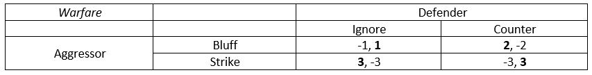
Warfare is expensive. In this game, the aggressor must choose between a costly strike or tactical bluff. While, striking is successful when the opponent is defenseless, it’s futile if the defender is prepared and ready to counter. Of course, the defender wants to counter if they believe the aggressor will strike. But if the aggressor is bluffing, the defender would rather commit resources elsewhere. Countering, after all, like striking, is expensive. We summarize the players, options, and payoffs in a game table as follows:
Game of pure conflict (tactical warfare)
Nash equilibrium in pure strategies
This variant of tactical warfare is a game of pure conflict. There is no Nash equilibrium in pure strategies. For any strategic profile in pure strategies, one player wants to change strategy. If, for example, the Aggressor believes the Defender will ignore, then the Aggressor will choose to strike. Anticipating this, however, the Defender will want to choose to counter. In this case, the Aggressor wants to Bluff, and so on, ad infinitum.
Nash equilibrium in mixed strategies
Remember, we have a Nash equilibrium when both players are using their best response, given what they believe the other will do. While the game above has no solution in pure strategies, there might be a Nash equilibrium in mixed strategies in which players randomize between their pure strategies. We call this a mixed strategy, much like playing a game of rock-paper-scissors.
To find this equilibrium, we search for a strategic profile in which both players are indifferent between their own strategies given the randomisation strategy the other is doing. Under such a profile, neither player has an incentive to change their mixed strategy (hence a Nash equilibrium!).
Mixed strategies
To find this solution, let’s first specify their randomisation strategies and expected payoffs.
Probability that Aggressor (A) chooses Bluff (B) or Strike (S):
1 = B + S
Probability that Defender (D) chooses Ignore (I) or Counter (C):
1 = I + C
Aggressor payoffs:
Aggressor’s expected payoff (AB) when it chooses Bluff:
AB = (-1 x I) + (2 x C)
Aggressor’s expected payoff (AS) when it chooses Strike:
AS = (3 x I) + (-3 x C)
Noting that 1 = I + C, the Aggressor is indifferent between Bluff and Strike when:
AB = AS
(-1 x I) + (2 x C) = (3 x I) + (-3 x C)
I = 5/9 and C = 4/9
It follows that: AB = AS = 1/3
Defender payoffs:
Defender’s expected payoff (DI) when it chooses Ignore:
DI = (1 x B) + (-3 x S)
Defender’s expected payoff (DC) when it chooses counter:
DC = (-2 x B) + (3 x S)
Noting that 1 = B + S, the Defender is indifferent between Ignore and Counter when:
DI = DC
(1 x B) + (-3 x S) = (-2 x B) + (3 x S)
B = 2/3 and S = 1/3
It follows that: DI = DC = -1/3
Nash equilibrium in mixed strategies
So, we have a Nash equilibrium in mixed strategies when: (1) the Defender randomises between Ignore with probability 5/9, and Counter with probability 4/9; and (2) the Aggressor randomises between Bluff with probability 2/3, and Strike with probability 1/3. The expected payoffs are 1/3 to the Aggressor, and -1/3 to the Defender.
This may not seem intuitive at first glance. But it’s important to remember that it is a Nash equilibrium when every player is using their best response to the best response of everyone else, and vice versa. This involved finding a mixed strategy that makes the other player indifferent between their pure strategies. And if everybody is playing such a mixed strategy, then nobody has an incentive to change their behaviour.
If, for example, the Aggressor were to choose another mix of probabilities, the Defender could earn a higher expected payoff by using a pure strategy (test this for yourself!). And if the Defender prefers to play a pure strategy, then the Aggressor’s best response is also a pure strategy – returning us to an unstable game of pure conflict.
Cardinal preferences and existence
In previous games of pure strategies, we assumed that players take actions to maximize their individual payoff. To make decisions with randomization, we make a similar but nuanced assumption: that players take actions to that maximize their expected payoff. And to estimate expected payoffs, we made an additional assumption: that the payoffs in the game table above were cardinal preferences. That is, the payoffs reflect the relative intensity of benefits to each player. Contrast this to simple games of pure strategies, where we only need to know the order of preferences to find a solution.
A Nash equilibrium in mixed strategies has several additional properties to keep in mind. Firstly, if the game consists of finite players with finite strategies, then there exists at least one Nash equilibrium in mixed strategies. Note that this is mixed strategies in a broader sense. It might mean a player playing some move with a probability of 1. Secondly, a Nash equilibrium in mixed strategies will never include strictly dominated strategies. It associates these strategies with a probability of zero. Intuitively, if an action is always inferior to another action, regardless of what others are doing, then it is never the best response.
Monitoring, deterrence, and mixing
It’s hard to imagine a business or state pursuing a mixing strategy. People dislike uncertainty. And leaving choice to chance seems unprofessional. Just imagine the backlash if a business executive pursued a strategy of randomisation. But there are tactical situations in which mixing strategies are viable. One popular example is in a game of monitoring and deterrence. Authorities cannot be everywhere at once to ensure compliance. The cost of mass surveillance is too large and politically untenable in many countries. Instead, authorities impose large penalties and randomise their inspections. If the expected cost of getting caught is sufficiently large, the randomisation strategy could deter misconduct. Good examples of this include random drug tests, ticket inspections, workplace safety audits, and so on.
Playing to your strengths and weaknesses
Mixing strategies provides some insight into competition as well. Let’s say you’re a football or basketball player who’s excellent at dribbling the ball to your right, but pretty poor at dribbling to your left. Defenders that know this will adjust more to your right, forcing you to your left more often. But if you improve your dribbling such that you are equally good at your left and right, then your opponent has to defend both positions equally. This, in turn, gives you more chances to dribble to your right. In this way, improving your weaknesses allows you to play more to your strengths. In games of strategic interdependence, players must re-evaluate their optimal mix of strategies when there is a change in relative payoffs.
Further reading
- Dominant strategies, dominated strategies and iterative deletion — Simplifying the game
- Nash equilibrium — A fundamental solution concept, and the hallmark of game theory
- The Game of Chicken — Your stake in nerves, ‘face’ and expectations
- The Prisoner’s Dilemma — An economic, political and evolutionary bastille
- Games of conflict and coordination — The tug-of-war of economic life
- Battle of the sexes: Mixing strategies in games of coordination and cooperation